Five ways to measure film thickness, and what each one really tells you

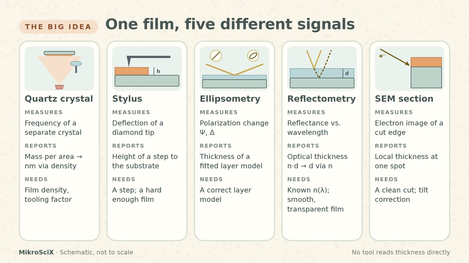
“How thick is this film?” sounds like a question with one answer. In a cleanroom it has at least five, because no instrument reads thickness directly. Each one measures a different signal (added mass, the height of a step, a change in polarization, an interference pattern or the image of a cut edge) and converts it into nanometres using its own assumptions.

This guide is for undergraduate and graduate students who use these tools, or soon will. For each method: what it actually measures, the equation behind it, one number you can check yourself, and the assumption that most often breaks.

1. Quartz crystal monitor: weighing a film you never touch

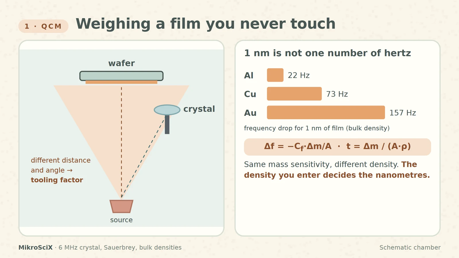
During evaporation or sputtering, a thin quartz crystal sits next to the wafer and vibrates at its resonance frequency, often around 6 MHz. As material lands on it, the frequency drops. The Sauerbrey relation converts that drop into mass per area:

Δf = −C_f · Δm / A

Dividing by the film density gives thickness: t = (Δm / A) / ρ.

Check it yourself. For a 6 MHz crystal, C_f ≈ 81.5 Hz per µg/cm². One nanometre of aluminium (2.70 g/cm³) is 0.27 µg/cm², about 22 Hz. One nanometre of gold (19.3 g/cm³) is about 157 Hz.

What breaks:

• Density. Thin films are often less dense than the bulk value. Enter a density 8 % too high and the monitor reads 8 % too thin.
• Geometry. The crystal and the wafer sit at different places in the vapour plume, so they collect different amounts. A tooling factor corrects this.
• Heavy loading. Sauerbrey assumes a thin, rigid, even layer; for thick films the Z-ratio correction is used.

Lab recipe. Deposit a reference film with a masked edge, measure the step with a profilometer, then set new tooling = old tooling × real thickness / monitor thickness. Monitor 100 nm, profilometer 85 nm: tooling goes from 100 % to 85 %.

2. Stylus profilometer: a diamond on a step

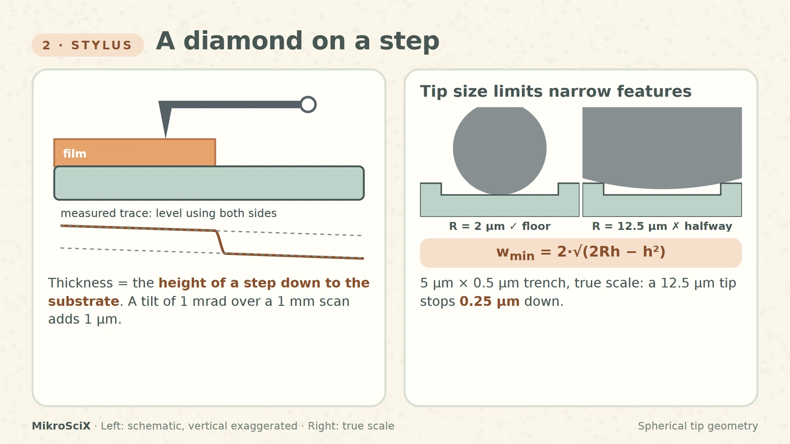
A diamond tip is dragged across the surface with a small force while its vertical deflection is recorded. Thickness is the height of a step from the film down to the substrate, so you need a step: a masked edge, a lift-off line or an etched window.

Vertical sensitivity is excellent: NIST calibrates steps of a few nanometres with ångström-level uncertainty. Lateral resolution is another story, because a round tip cannot follow a narrow, deep trench. A tip of radius R reaches the floor of a trench of depth h only if the trench is wider than:

w_min = 2 · √(2Rh − h²)

Check it yourself. For a 0.5 µm deep trench, a 2 µm tip needs about 2.6 µm of width; a 12.5 µm tip needs about 7 µm. In a 5 µm trench the blunt tip stops 0.25 µm down and reports half the real depth.

What breaks:

• Leveling. A tilt of 1 mrad over a 1 mm scan adds 1 µm. Fit the baseline on flat regions on both sides of the step.
• The reference level. Over-etching into the substrate adds to the “film”; residue under it subtracts.
• Soft films. Resists and polymers can be scratched: lower the force or use an optical method.

3. Spectroscopic ellipsometry: thickness from polarization

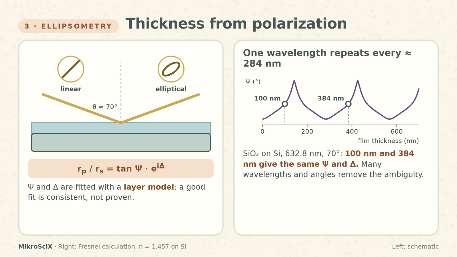
Polarized light hits the sample at a steep angle, often near 70°. Reflection turns linear polarization into elliptical, and the instrument records the change as two angles, Ψ and Δ, at many wavelengths:

r_p / r_s = tan Ψ · e^(iΔ)

Ψ and Δ are not thickness. Thickness comes from fitting a layer model (substrate, film thickness, optical constants) until the calculated curves match the measured ones. A good fit means the model is consistent with the data, not that it is the only possible answer.

Check it yourself. For SiO₂ on silicon at 632.8 nm and 70°, Ψ and Δ repeat every λ / (2√(n² − sin²θ)) ≈ 284 nm. A single-wavelength measurement cannot tell 100 nm from 384 nm. Spectroscopic data and several angles remove the ambiguity.

What breaks:

• A missing layer in the model: native oxide, an interface layer or roughness.
• Very thin films: thickness and refractive index trade off. Fix n to a known value and fit only d.
• Non-uniform films inside the measurement spot.

4. Spectral reflectometry: counting fringes

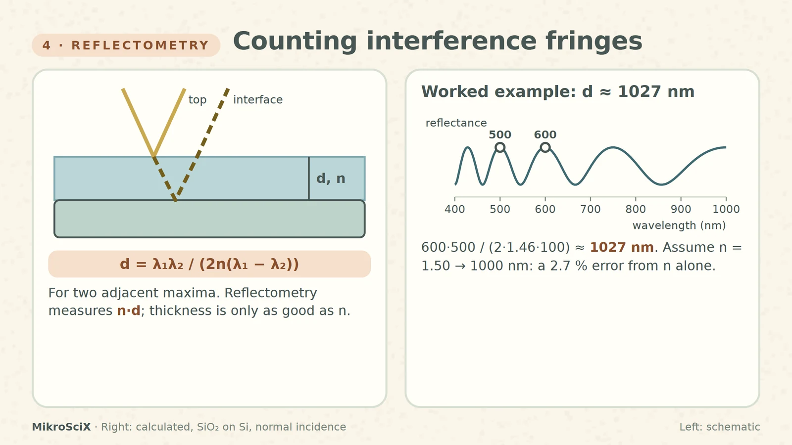
White light hits a transparent film at normal incidence. Light reflected from the top surface and from the film–substrate interface interferes, so the reflectance spectrum oscillates. The spacing of the oscillations encodes the optical thickness n·d. For two adjacent maxima at λ₁ > λ₂:

d = λ₁λ₂ / (2n(λ₁ − λ₂))

Check it yourself. SiO₂ (n ≈ 1.46) with maxima at 600 nm and 500 nm gives d = 600·500 / (2·1.46·100) ≈ 1027 nm. Assume n = 1.50 instead and you get 1000 nm: a 2.7 % error from the refractive index alone.

What breaks:

• The refractive index and its dispersion over the wavelength range.
• Very thin films show less than one fringe in the spectrometer window, so the fit leans harder on the model.
• Rough or opaque films, and a poor reference measurement.

Its strength is convenience: it is contactless, and scanning the spot can map a whole wafer.

5. SEM cross-section: cut it and look

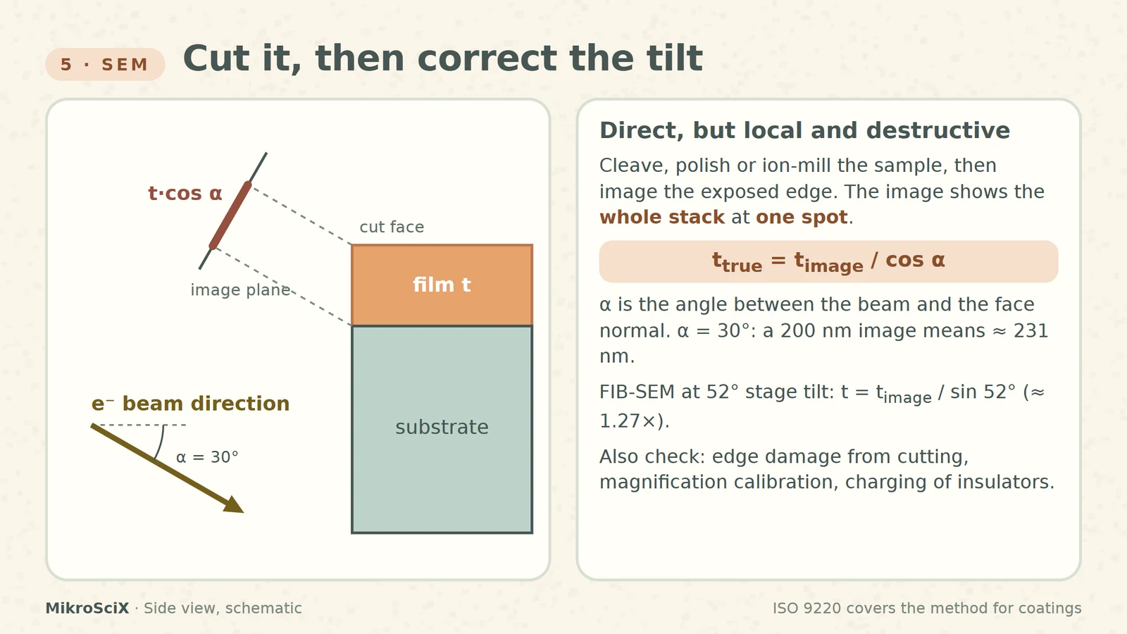
Cleave, polish or ion-mill the sample, then image the exposed edge in a scanning electron microscope. You see the whole stack, interfaces included, directly. The price: the method is destructive and the result is local, one place on one sample. ISO 9220 describes this approach for coating thickness.

Check it yourself. If the beam meets the cut face at an angle α from its normal, the image shortens vertical distances by cos α, so t_true = t_image / cos α. At α = 30°, a film that looks 200 nm is about 231 nm. In a FIB-SEM with the stage at 52°, a milled face perpendicular to the surface needs t_image / sin 52°, about 1.27×.

What breaks:

• Representativeness. One section is not the whole wafer.
• The edge. Cleaving can smear ductile metals or tear polymers; polishing can round edges.
• The scale. Magnification calibration, charging of insulating films, and deciding where a blurred interface really is.

How to choose

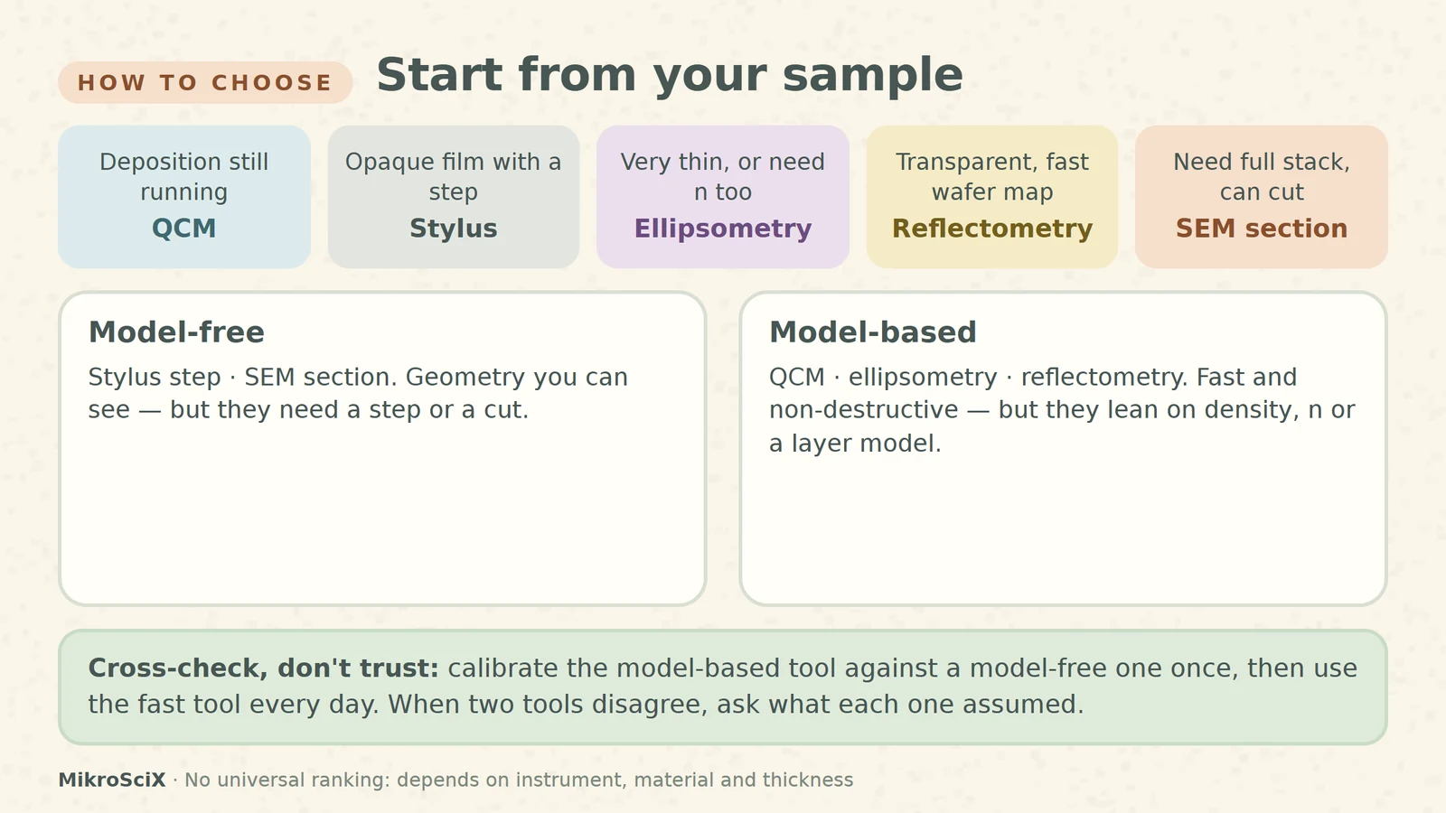
Start from your sample, not from the instrument you happen to know.

• Deposition still running? Quartz crystal monitor, calibrated afterwards.
• Opaque film with a clean step? Stylus profilometer.
• Very thin film, or optical constants needed too? Ellipsometry.
• Transparent, smooth film and a wafer map? Reflectometry.
• Full stack at one feature, and the sample can be sacrificed? SEM cross-section.

There is no universal ranking: range, precision and speed depend on the instrument, the material, the thickness and the preparation.

The habit that matters most

Pair a model-free method (a step or a section) with a model-based one (the crystal monitor or an optical method). Calibrate once, then use the fast method every day. When two results disagree, don't average them: ask what each one assumed, whether density, reference level, optical model or section location.

Every thickness number is a measurement plus a model. Know which model you are trusting.

Try it yourself

1. A 6 MHz monitor drops 440 Hz while depositing aluminium. What is the thickness on the crystal?
2. A polymer film (n = 1.55) shows adjacent reflectance minima at 650 nm and 550 nm. How thick is it?
3. A 5 µm-radius tip scans a trench 1 µm deep and 5 µm wide. Does it reach the floor?

Answers: (1) 440 / 81.5 ≈ 5.4 µg/cm², about 20 nm. (2) 650·550 / (2·1.55·100) ≈ 1153 nm. (3) No: it needs about 6 µm of width.