Why your solar cell reads negative current on an SMU, and four other things the instrument is telling you

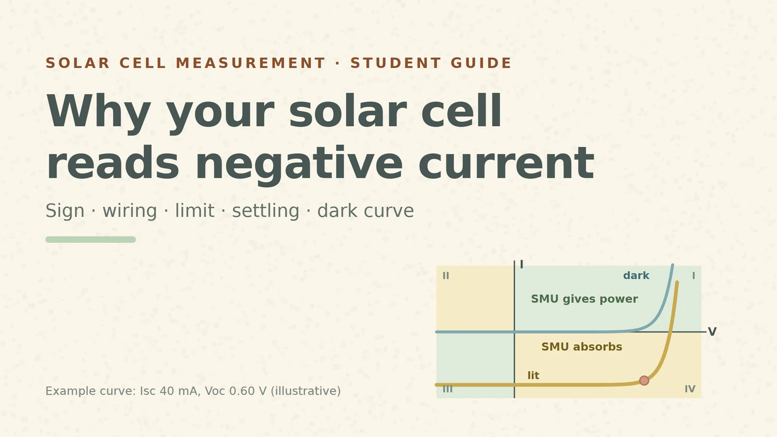
You clip a small solar cell under a lamp, connect it to a source-measure unit (SMU), start a voltage sweep and look at the first reading: +0.45 V, −39.1 mA. A minus sign on the current. Many students rewire the cell at this point. Don't: the minus sign is the instrument telling you, correctly, that the cell is producing power.

This guide follows what you actually see on the screen, step by step. Each section gives the rule, a number you can check yourself, and what breaks. All numbers come from one invented example cell: short-circuit current Isc = 40 mA, open-circuit voltage Voc = 0.60 V, about 36.7 mA at 0.50 V (the same example as our solar-cell-parameters video). They are teaching values, not measurements.

1. The minus sign: four quadrants, two jobs

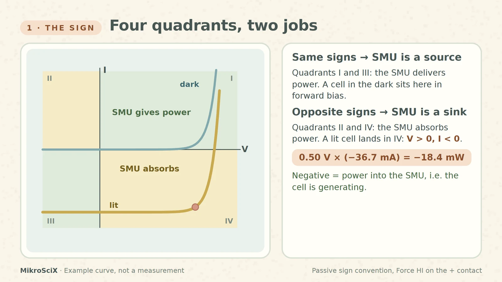
An SMU can work in all four quadrants of the V–I plane. In quadrants I and III, voltage and current have the same sign: the SMU is a source and delivers power. In quadrants II and IV the signs are opposite: the SMU is a sink and absorbs power, as it does when another source forces current into it [S2].

A lit cell is such a source. When the SMU holds a voltage between 0 V and Voc, the cell pushes current out of its positive contact and into the SMU. The instrument counts current flowing out of its own HI terminal as positive, so it reports V > 0 and I < 0: quadrant IV. Keithley's solar-cell note says exactly this: because the SMUs can sink current, the illuminated curve passes through the fourth quadrant and power is extracted from the device [S1].

Check it yourself. At 0.50 V the example cell gives 36.7 mA. The SMU reads +0.50 V and −36.7 mA, so the power into the SMU is V × I = −18.4 mW. The sign says "absorbed": the cell delivers +18.4 mW.

What breaks:

• Flipping the leads to "fix" the sign. Then the cell's negative contact sits on HI and the sweep from 0 V to +Voc no longer runs along the generating part of the curve. Keep Force HI on the positive contact and flip the plot instead: the note shows how to invert the graph about the voltage axis [S1].
• Forgetting the sink limits. Sinking is still power the SMU must dissipate; it has its own source and sink boundaries [S2].

2. The voltage that is a few percent low: two wires versus four

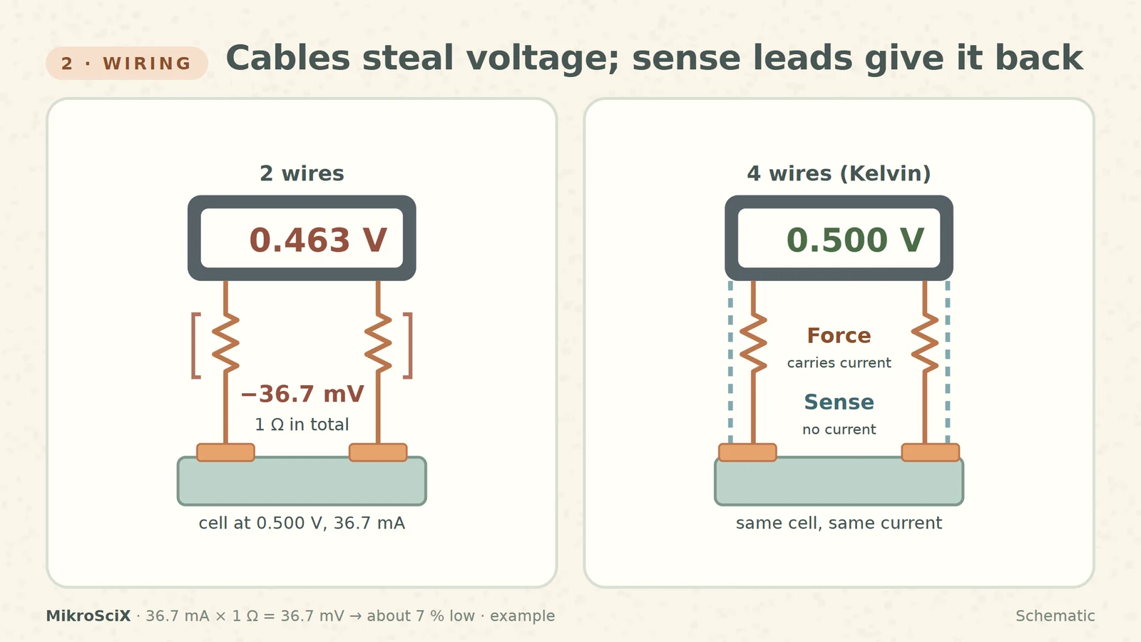
Current has to travel through the cables, and every cable has resistance. If the same two wires carry the current and measure the voltage, the reading includes the voltage drop along the cables. In a four-wire (Kelvin) connection the force pair carries the current and a separate sense pair, touching the cell's contacts, measures the voltage; the sense leads compensate for the lead resistance [S1][S2].

Check it yourself. Round numbers first: 40 mA through 1 Ω of cable drops 40 mV. With the example curve at 0.50 V, the current is 36.7 mA, so the drop is 36.7 mV. A generating cell drives that current through the cables, so the far end is lower: a two-wire SMU reads 0.463 V instead of 0.500 V, about 7 % low. The power you compute drops from 18.4 mW to 0.463 × 36.7 ≈ 17.0 mW.

What breaks:

• Sense leads clipped to the cable instead of the cell. They only exclude what lies between their two contact points; land them on the cell's own contacts.
• Thinking the error is constant. The drop is current × resistance, so it is largest where the current is largest: on the flat, high-current part of the curve.

3. The flat shelf: a current limit below Isc

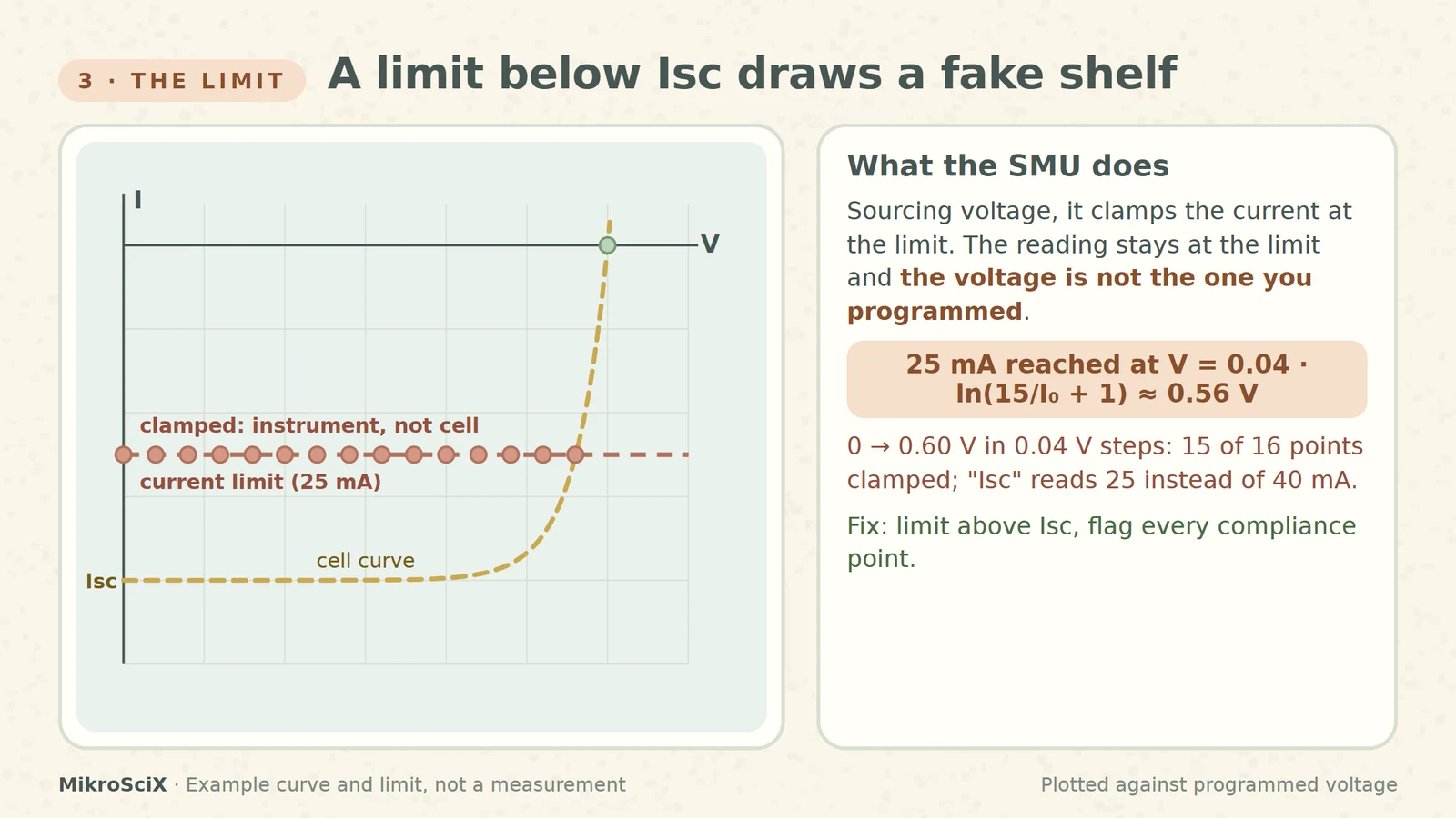
Every SMU has a protection limit called compliance. When it sources voltage, current is clamped at the compliance value. The manual is explicit about what happens then: the instrument keeps measuring, the current reading stays at the limit, and the voltage is not the programmed value [S2].

For a solar cell this has a striking consequence. Near 0 V the cell wants to push its full short-circuit current. If the limit is below Isc, the SMU cannot hold the low voltages: the cell's voltage rises until its current falls to the limit.

Check it yourself. Set a 25 mA limit on the 40 mA example cell. The cell gives exactly 25 mA at V = 0.04 V × ln(15 / I0 + 1) ≈ 0.56 V, with I0 = 40 mA / (e¹⁵ − 1). Every step programmed below 0.56 V reads −25 mA, while the cell actually sits near 0.56 V. Sweep 0 to 0.60 V in 0.04 V steps and 15 of the 16 points are clamped. Plotted against the programmed voltage, you get a flat shelf and an "Isc" of 25 mA instead of 40 mA, 37.5 % low.

What breaks:

• Reading the shelf as a property of the cell. It is the instrument. Flag compliance points (most software can report or stop on them [S2]) and never fit them.
• Setting the limit by habit. There is no universal value: choose it above the cell's current and inside the instrument's range. The 4200 note also suggests reducing the cell area if its current exceeds what the SMU can sink [S1].

4. The staircase: step, settle, read

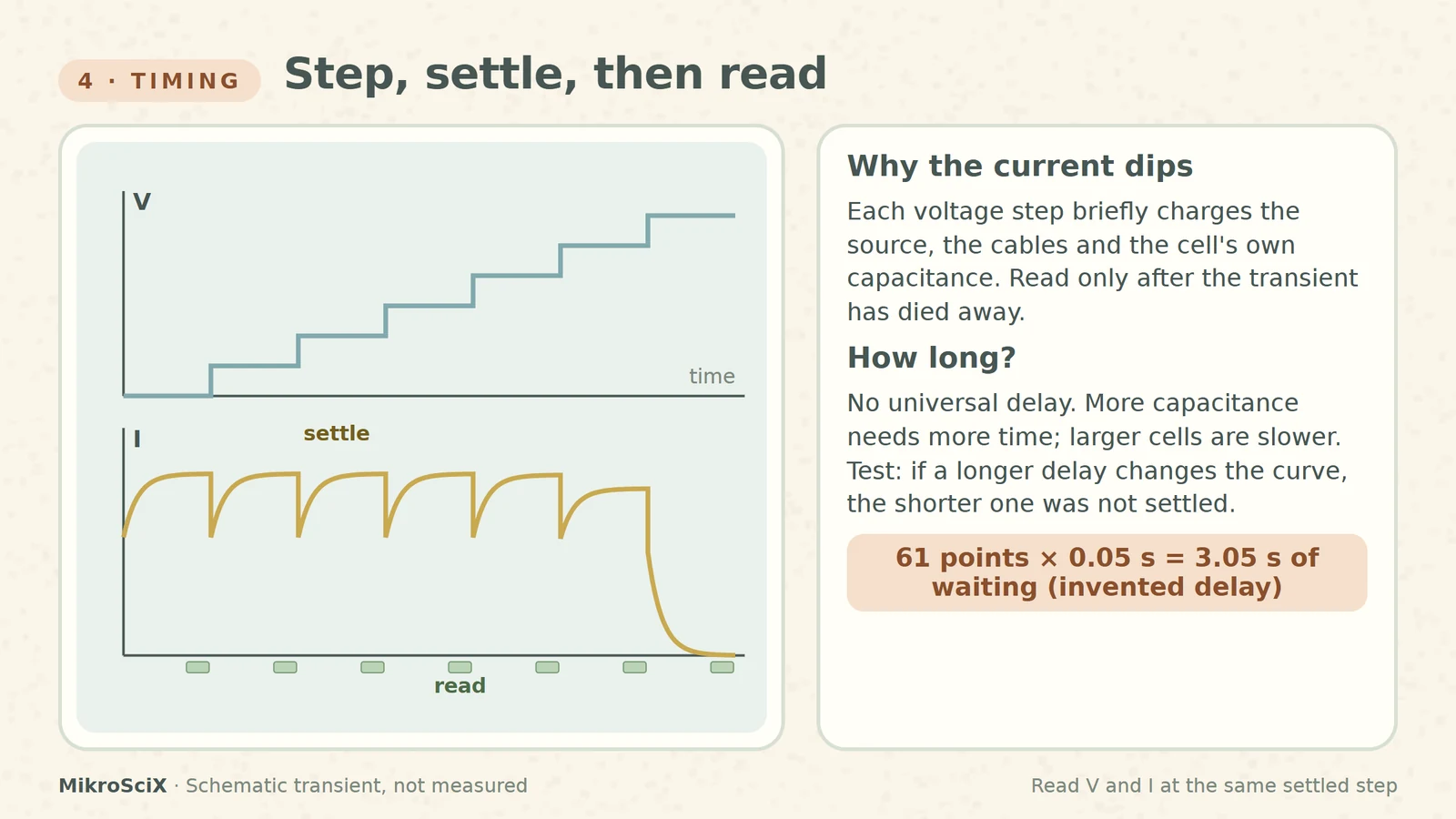
A forward sweep steps the voltage from 0 V toward Voc and measures current at each step [S1][S2]. After each step the current needs time to settle: the source, the cables and the cell's own capacitance all respond. The SMU's delay settings exist for this; more capacitance at the output needs more settling time [S2], and larger cells have larger capacitance, which can mean a long settling time [S1].

Check it yourself. The waiting adds up: with an invented 50 ms delay per step, 61 points spend 61 × 0.05 s = 3.05 s just waiting, before any integration time. Halve the points or the delay and the sweep is faster, but only the second choice risks unsettled readings.

What breaks:

• Reading inside the transient. The point lands off the true curve. Voltage and current must be read together, at the same settled step.
• Copying someone else's delay. No single delay is correct; it depends on the cell, cables and range. Test it: if a longer delay changes the curve, the shorter one was not settled.

5. The dark curve: the same cell, now just a diode

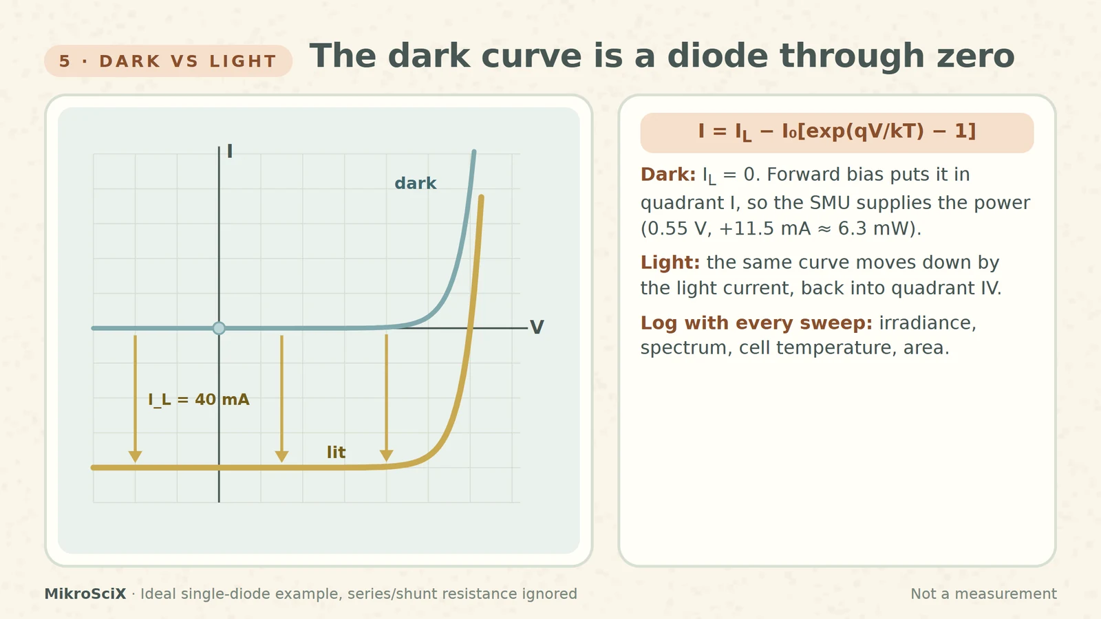
The ideal cell equation is I = IL − I0[exp(qV/kT) − 1]: the light-generated current minus the diode current [S3]. Switch the light off and IL = 0. What remains is a diode: the curve passes through zero and, in forward bias, voltage and current have the same sign. That is quadrant I, where the SMU supplies the power. Switch the light on and the whole curve moves down by the light current, back into quadrant IV.

Check it yourself. In the dark at +0.55 V the example diode carries I0 × (e^13.75 − 1) ≈ 11.5 mA, so the SMU reads +0.55 V, +11.5 mA and supplies about 6.3 mW. Under light, the same voltage reads 40 − 11.5 = 28.5 mA out of the cell, so the SMU sees −28.5 mA.

Because the curve depends on light and temperature (T sits inside the diode term), a result means little without its conditions. NREL reports performance against a reference temperature, total irradiance and spectrum, measures irradiance and cell temperature with each curve, and treats the device area as crucial [S4]. Log all of them with every sweep.

6. Without an SMU: electronic loads

An electronic load plus meters can also trace the curve, but it must reach 0 V to capture Isc. Keysight's note on its N3300 series is candid: performance degrades below 3 V and at 0 V no current can flow into the load; the fix is a boost power supply in series so the load always works at 3 V or more [S5]. Some loads are fine near zero volts, some are not: check the low-voltage specification before you trust the short-circuit end.

Check it yourself. A single cell spans 0 to 0.60 V. With a 3 V boost supply in series, the load sees about 3.0 to 3.6 V, inside its working range, while the cell still sweeps from short circuit to open circuit.

A five-line checklist before you press "run"

1. Sign: Force HI on the positive contact; expect V > 0, I < 0 under light.
2. Wiring: four wires, sense on the cell's own contacts.
3. Limit: compliance above Isc; flag any clamped point.
4. Timing: a delay you have tested, and the same in every comparison.
5. Record: irradiance, spectrum, cell temperature, area, sweep range and timing, limits.

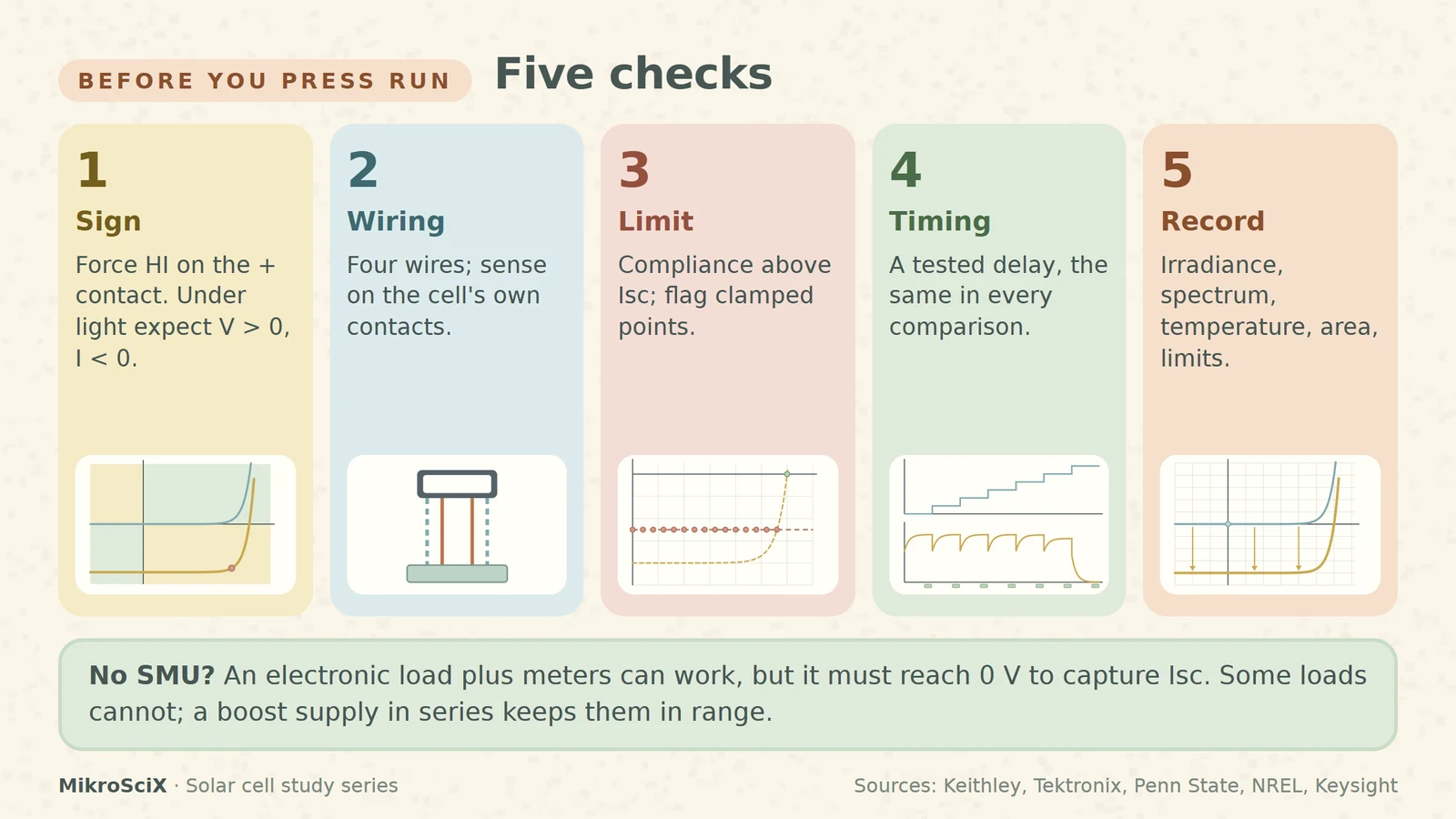
A solar cell on an SMU is two power sources talking. Read the sign, sense at the cell, keep the limit out of the way, let every step settle, and write down the light.

Try it yourself

1. The SMU shows +0.45 V and −39.1 mA. Is the cell generating, and how much power? Yes: opposite signs, quadrant IV. P = 0.45 V × 39.1 mA ≈ 17.6 mW delivered by the cell.
2. Two-wire, 0.5 Ω of total cable, true cell voltage 0.50 V (36.7 mA). What does the SMU read? Drop = 36.7 mA × 0.5 Ω ≈ 18 mV, so about 0.482 V.
3. Limit raised to 30 mA on the example cell. Up to which voltage are points clamped? V = 0.04 × ln(10 / I0 + 1) ≈ 0.54 V.
4. A dark sweep at +0.55 V reads +11.5 mA. Who supplies the power? Same signs, quadrant I: the SMU supplies about 6.3 mW.