Doomsday, 13 November 2026: the 1960 equation that 'predicted' the end, and why it broke

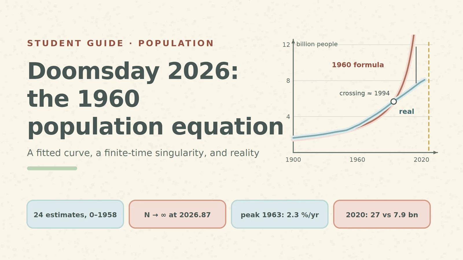
Every few years a headline announces that "scientists predicted the end of the world" for a specific date. For 13 November 2026 the story is real in one sense: a peer-reviewed paper with that date in its title appeared in Science on 4 November 1960. Its authors, Heinz von Foerster, Patricia Mora and Lawrence Amiot of the University of Illinois, did not predict a catastrophe. They fitted a formula to the history of the world population and pointed out where that formula ends.

This guide walks through the formula step by step: what it fits, why it reaches infinity on a finite date, how that differs from exponential growth, what happened after 1960, and why a curve that fits the past is not a forecast. Each part has a number you can check yourself.

1. The fit: 24 estimates, one curve

The authors collected 24 independent estimates of the world population, from the year 0 to 1958, roughly a hundred generations. They removed estimates that only copied each other and fitted the rest by least squares to a three-parameter law:

N(t) = K / (t₀ − t)^k, with K = 1.79 × 10¹¹, k = 0.99, t₀ = A.D. 2026.87 ± 5.5 years

The root-mean-square deviation of the estimates from the curve was about 7 %. The date t₀ is the "doomsday": as t approaches t₀ the denominator goes to zero and N goes to infinity. The fraction 0.87 of the year 2026 falls in mid-November, and the authors dated it to Friday, 13 November.

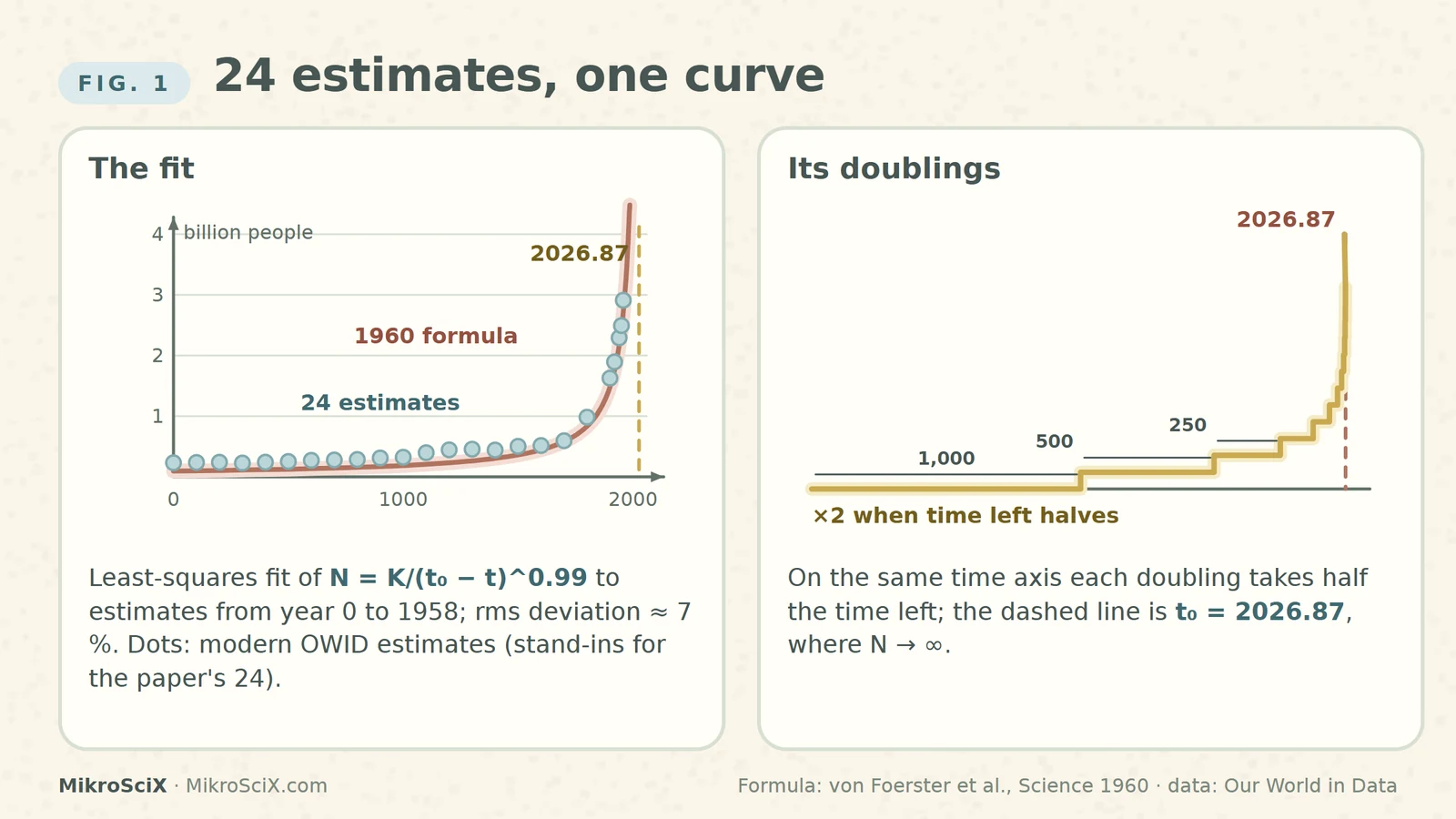
The dots in our figures are modern estimates for 24 years between 0 and 1958 from Our World in Data, used as stand-ins for the paper's own 24 values, which are only shown on a log chart in the original. They follow the same curve closely.

Check it yourself: for 1960 the formula gives N = 179 billion / (66.87)^0.99. Since 66.87^0.99 ≈ 64.1, N ≈ 2.79 billion. The modern estimate for 1960 is 3.02 billion, about 8 % higher, which is within the scatter the authors reported.

What breaks: nothing yet. Over two thousand years the curve really did describe the data well. That is exactly what made the paper famous, and exactly what makes it a good lesson.

2. The idea behind it: growth that feeds itself

In ordinary population models each person contributes a fixed growth rate, so the total grows exponentially. Von Foerster and colleagues argued that humans are different: people who communicate form coalitions, build better technology and make their environment less hostile. So the growth rate itself rises with the population. More people, faster growth, even more people.

Writing the growth rate as a power of N and integrating gives the law above. Because k is almost exactly 1, the rule becomes very simple: the population is inversely proportional to the time left until t₀. The physicist Sergey Kapitza later described the same history with a growth rate proportional to N², which is the same hyperbola written as a differential equation: dN/dt = N²/C has the solution N = C/(t₀ − t).

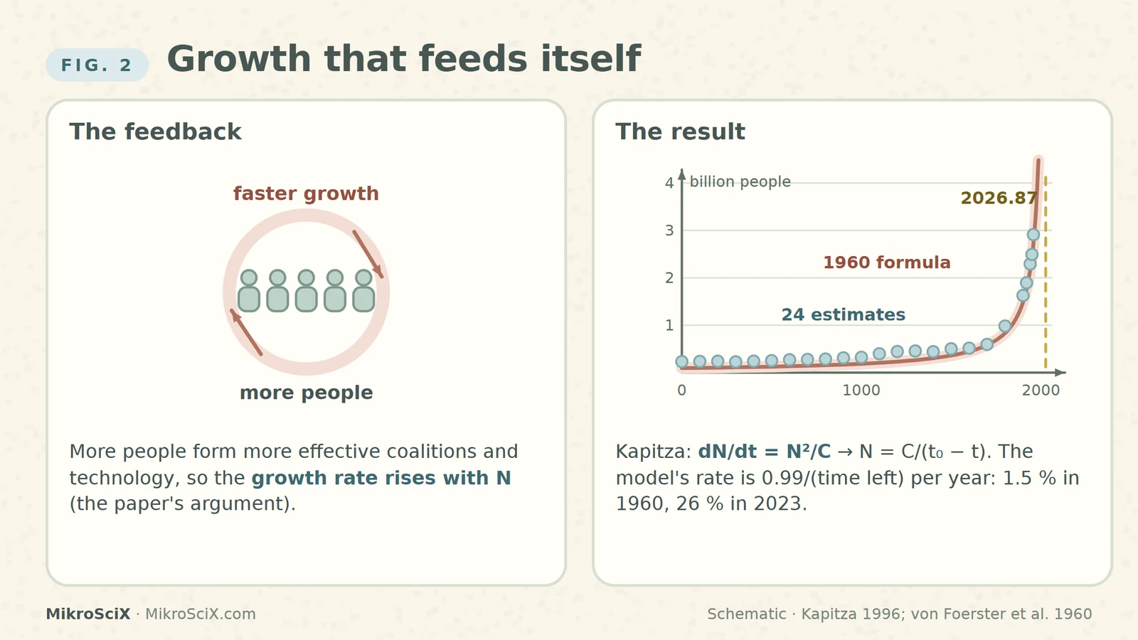
Check it yourself: the model's own growth rate is 0.99 / (time left) per year. In 1960 that is 0.99 / 66.87 ≈ 1.5 % per year. In 2023 it would be 0.99 / 3.87 ≈ 26 % per year.

What breaks: a rate that keeps rising has no ceiling. Any real feedback loop runs into limits of a different kind, and that is where the next sections go.

3. Hyperbolic vs exponential: doublings that speed up

The clearest way to see the difference is to count doublings. Exponential growth at a constant rate r doubles on a fixed clock, every ln 2 / r years: at 2 % per year that is every 35 years, forever. It becomes infinite only after infinite time.

In the 1960 law, N ∝ 1/(time left). The population doubles whenever the time left halves. Starting in the year 1, with about 2,026 years left, the first doubling takes about 1,000 years (to around 1021), the next about 500 (to around 1527), then 250 (around 1779), 125 (around 1904), 61 (around 1966), 30 (around 1996), 15, 7.5, 3.7 … Each doubling takes half as long as the previous one, so infinitely many doublings fit before one finite date.

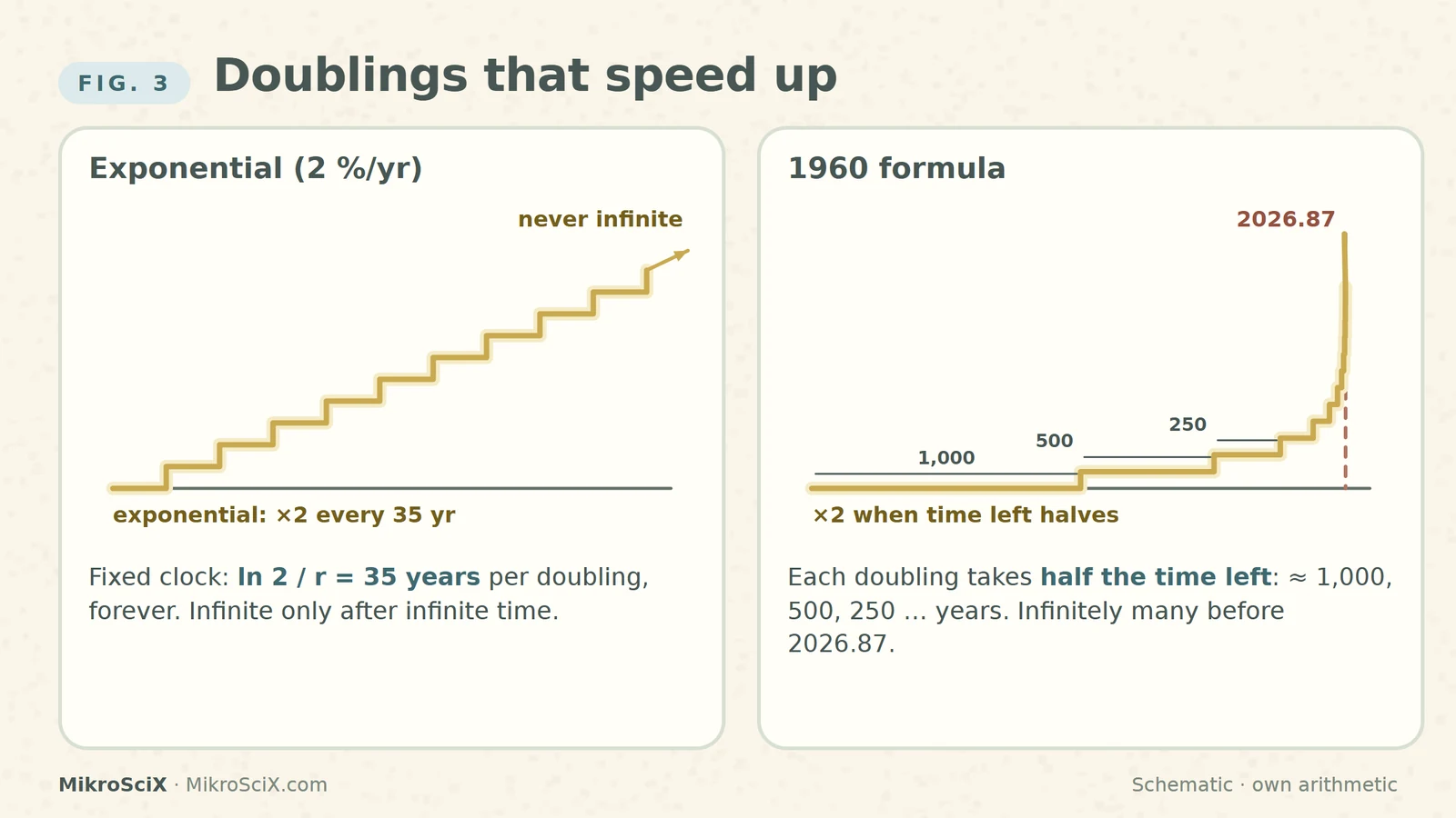
Check it yourself: with k = 0.99 each doubling multiplies the time left by 2^(−1/0.99) ≈ 0.4965. From 1966 (61 years left) one doubling brings you to 61 × 0.4965 ≈ 30 years left, the year 1996.5. Exponential growth at 2 %: ln 2 / 0.02 = 34.7 years per doubling.

What breaks: the words "exponential growth" are often used for anything that grows fast. The doomsday curve is faster than any exponential: it is a finite-time singularity.

4. Why it looks like a straight line on the right chart

If N = K/τ^k, with τ = t₀ − t, then log N = log K − k · log τ. On a chart with logarithmic axes for both the population and the time left, the whole two-thousand-year history becomes a straight line with slope −0.99. This is how the original paper plotted its data, and it explains why the fit looked so convincing: one straight line through points spanning more than a factor of ten in population.

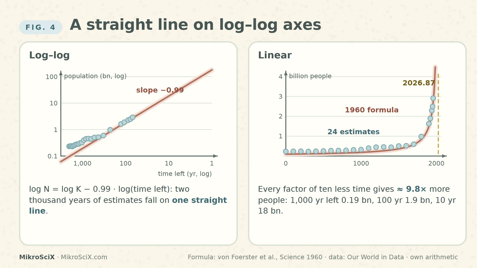
Check it yourself: 1,000 years left gives 179 / 1000^0.99 ≈ 0.19 billion; 100 years left gives about 1.9 billion; 10 years left gives about 18 billion. Every factor of ten less time means about 9.8 times more people.

What breaks: a straight line on a log–log chart is easy to extend with a ruler. The authors noted that they had to extrapolate only about 4 % beyond their last observation (68 years after a record of almost two thousand) and could "predict doomsday within approximately 10 years"; Charlemagne, they joked, could have done it within 300 years. But on this curve those last 68 years contain infinitely many doublings: a short step in time is an endless step in the mechanism.

5. What actually happened

The real world broke away from the curve in two stages. First the growth rate: world population growth peaked at about 2.3 % per year in 1963 and has fallen since, to 0.9 % in 2023, as families became smaller across the world. Demographers call this the demographic transition, and Kapitza dated its global start to about 1965. The model, by contrast, demands a rate that rises without limit.

Second the count. Because the formula slightly under-predicted the 1960s to 1980s, the real population stayed above the curve for a while. A comparison of the formula with modern data puts the crossing between 1993 and 1995; a Conversation article by the historian Alan MacEachern says the predictions looked accurate "until around 1993". After that the curve shoots away.

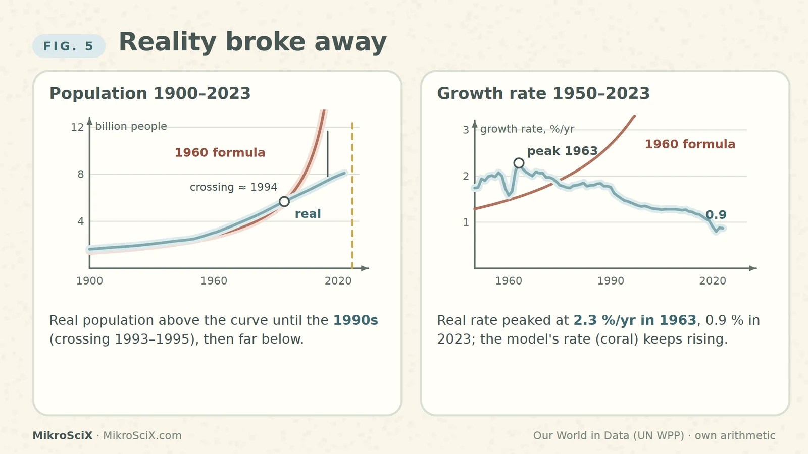
Check it yourself: formula for 1993: 179 / 33.87^0.99 ≈ 5.47 billion; modern estimate 5.59 billion (2 % above). Formula for 1995: 5.81 billion; estimate 5.76 billion (1 % below). The crossing is between the two.

What breaks: secondary sources disagree whether the model "failed in the 1960s" or "in 1993". Both are right about different quantities: the rate broke first, the count followed thirty years later.

6. The pitfall: a fit is not a forecast

For 2020 the formula gives about 27 billion people. The real count was 7.9 billion, so the curve is off by more than a factor of three, and the gap grows every year until t₀. The United Nations now projects that the world population, 8.2 billion in 2024, will peak at about 10.3 billion in the mid-2080s and then slowly decline.

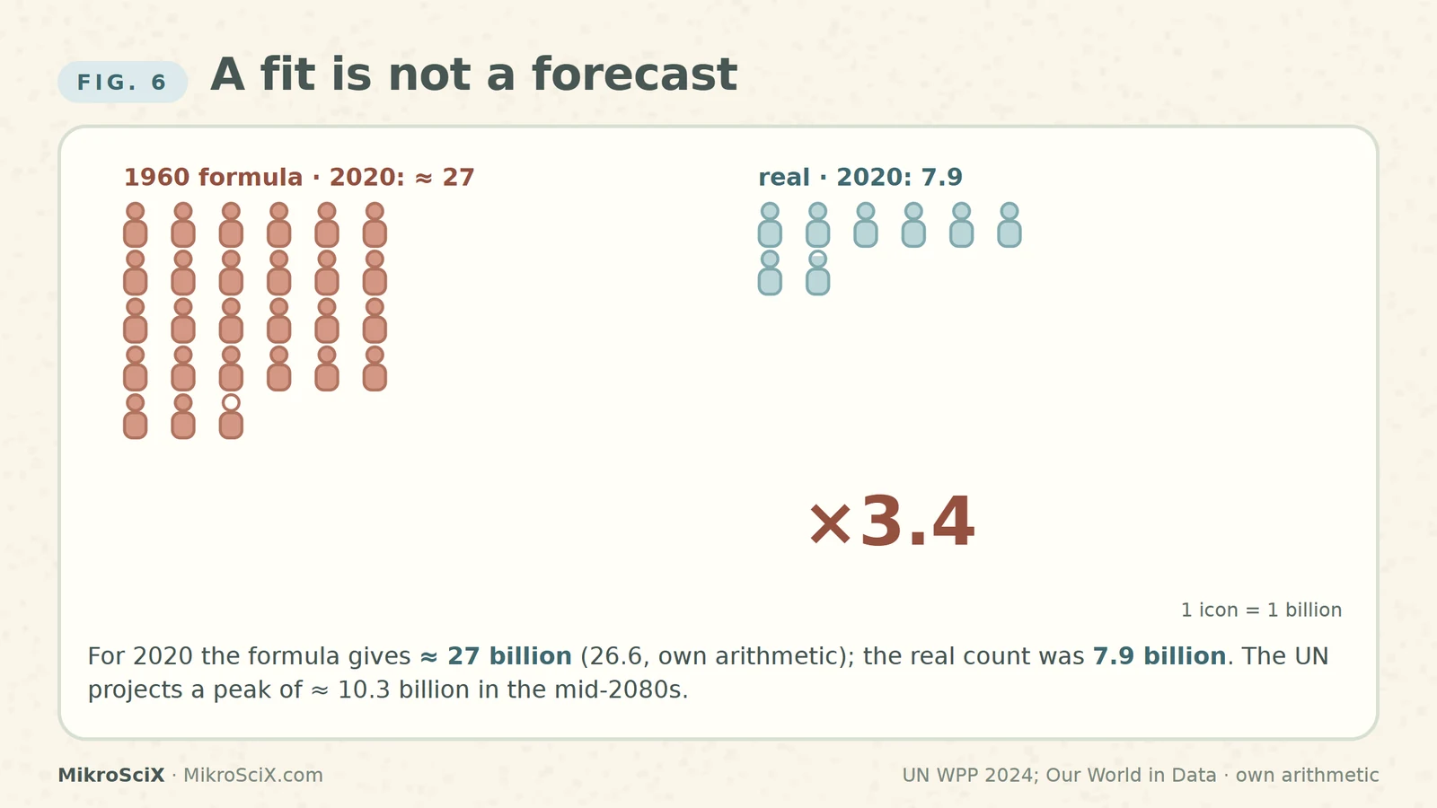
Check it yourself: 2026.87 − 2020 = 6.87 years left; 6.87^0.99 ≈ 6.74; 179 / 6.74 ≈ 26.6 billion (28.6 billion if you take mid-2020). 26.6 / 7.89 ≈ 3.4.

A curve that fits the past well is a description of the past. Extending it is an assumption that the mechanism stays the same.

The authors knew this. Their paper ends not with doom but with a proposal: since nobody wants to shorten lives, humanity would have to control fertility, cutting the birth rate to about half, to families of just over two children. Their famous line, that our great-great-grandchildren "will not starve to death; they will be squeezed to death", was a warning about what happens if nothing changes. Something did change.

How to read the next "scientists predicted the end" headline

Find the model. Is the date a forecast, or the point where a fitted formula becomes infinite?
Find the mechanism. What assumption makes the curve explode, and is there a reason it must keep holding?
Find the distance. How far beyond the last data point is the claim? Uncertainty grows fastest exactly where singular curves turn steep.
Find the original. The 1960 paper is often attributed to "Harvard"; its authors were at the University of Illinois.

Try it yourself

In which year does the 1960 formula reach 10 billion people? Answer: (2026.87 − t)^0.99 = 17.9, so 2026.87 − t ≈ 18.4 years, t ≈ 2008. The real population passed 8 billion only around 2022.
At the 1963 peak rate of 2.3 % per year, how long would one doubling take? Answer: ln 2 / 0.023 ≈ 30 years.
How many doublings does the formula fit between 1958 and 2026.87? Answer: infinitely many; the time left halves without end.
On a log–log chart, what happens to the population when the time left drops from 100 to 10 years? Answer: it grows by 10^0.99 ≈ 9.8 times, from about 1.9 to about 18 billion.