Quantum efficiency: which colours a solar cell turns into current, and how to read the curve

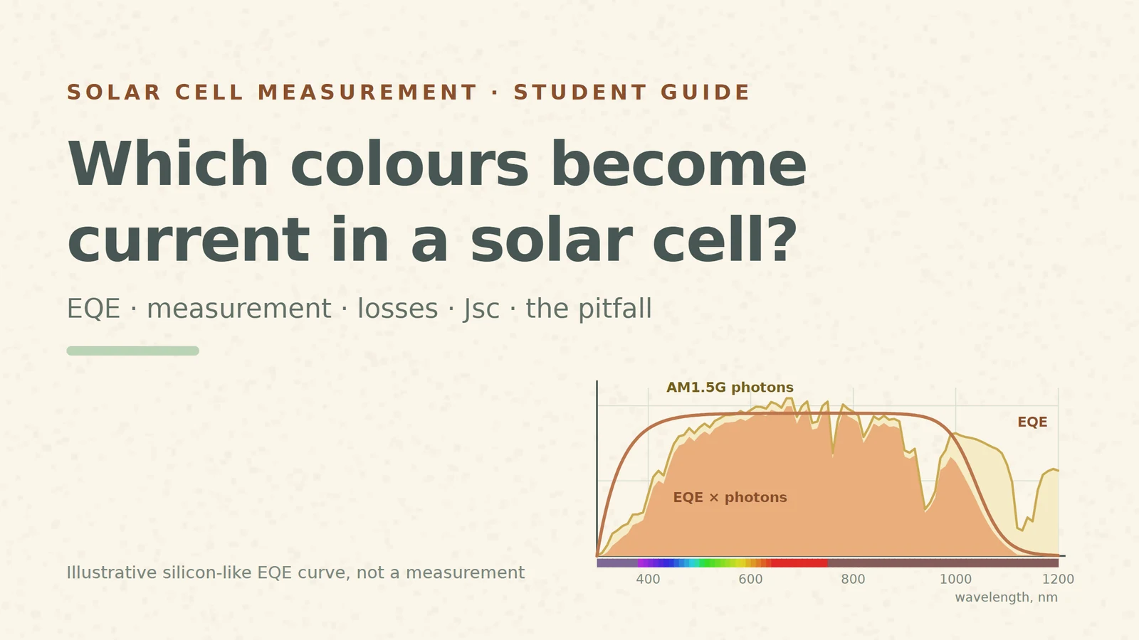
Put a solar cell under a lamp and measure its short-circuit current: one number, say 38 mA/cm². It hides a lot. Was the blue part of the light wasted at the surface? Did the red light run out of silicon before it was absorbed? Is the top layer simply reflecting too much? To answer, you have to light the cell with one colour at a time and count. That count is the quantum efficiency.

This guide uses one illustrative curve throughout: a silicon-like external quantum efficiency (EQE) whose shape follows the textbook picture [S1]. It is a teaching example, not a measured cell. Where we turn it into a current, we use the real ASTM G-173 reference spectrum [S6] and show our own arithmetic.

1. Count electrons per photon

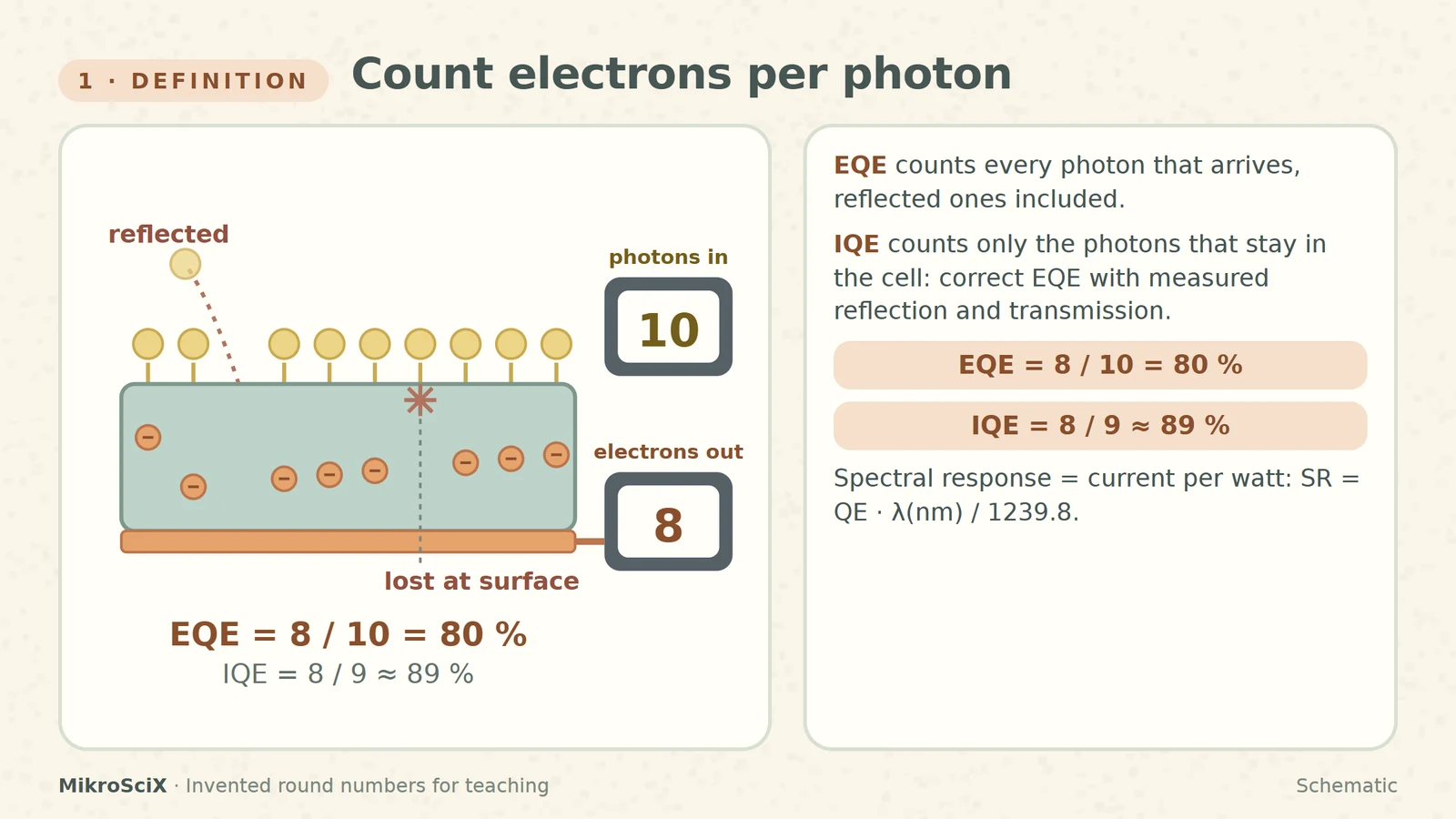
The quantum efficiency at a wavelength is the number of carriers the cell collects divided by the number of photons of that wavelength that arrive [S1]. If every photon of a colour is absorbed and every carrier it makes reaches the contacts, QE at that colour is 1 (100 %). Below the band gap it is 0: those photons are not absorbed at all.

There are two versions. The external quantum efficiency counts every photon that arrives, including those reflected off the surface or transmitted through the cell. The internal quantum efficiency counts only the photons that actually stayed in the cell. Measure the reflection and transmission, correct EQE for them, and you get IQE [S1][S5]. IQE is therefore always at least as high as EQE.

Check it yourself. Ten photons of one colour arrive. One is reflected, one is absorbed right at the surface and its carriers recombine, eight are collected. EQE = 8/10 = 80 %. Leave out the reflected photon: IQE = 8/9 ≈ 89 %. (Invented round numbers; a real measurement gives fractions.)

A close relative is the spectral response (or responsivity): current per watt of light instead of electrons per photon. Because a photon's energy depends on its colour, the two convert with SR (A/W) = QE · λ(nm) / 1239.8 [S2]. At 550 nm our example EQE is 0.946, so SR = 0.946 × 550 / 1239.8 ≈ 0.42 A/W.

What breaks. Calling a curve "IQE" without measuring reflection and transmission. And in thin cells, light that passes straight through is an EQE loss that IQE hides.

2. How it is measured: one colour at a time

The classic system is simple in principle [S3]. A broadband lamp is chopped and then filtered or diffracted by a monochromator into a narrow band of wavelengths. That band goes, one after another, to two places:

• A calibrated detector of known responsivity (a pyroelectric radiometer or a calibrated semiconductor detector) measures the beam's power, and so its photon rate [S3][S5].
• The cell, usually held at zero voltage (short circuit), delivers a current. A lock-in amplifier locked to the chopper frequency picks out exactly the current made by the chopped beam and ignores room light [S3].

Current divided by power gives the responsivity, which converts to electrons per photon. Step the monochromator and the curve appears, point by point. Options: a steady bias light brings the cell closer to its operating conditions under sunlight, and a voltage bias is needed for some devices, such as multijunction cells [S3].

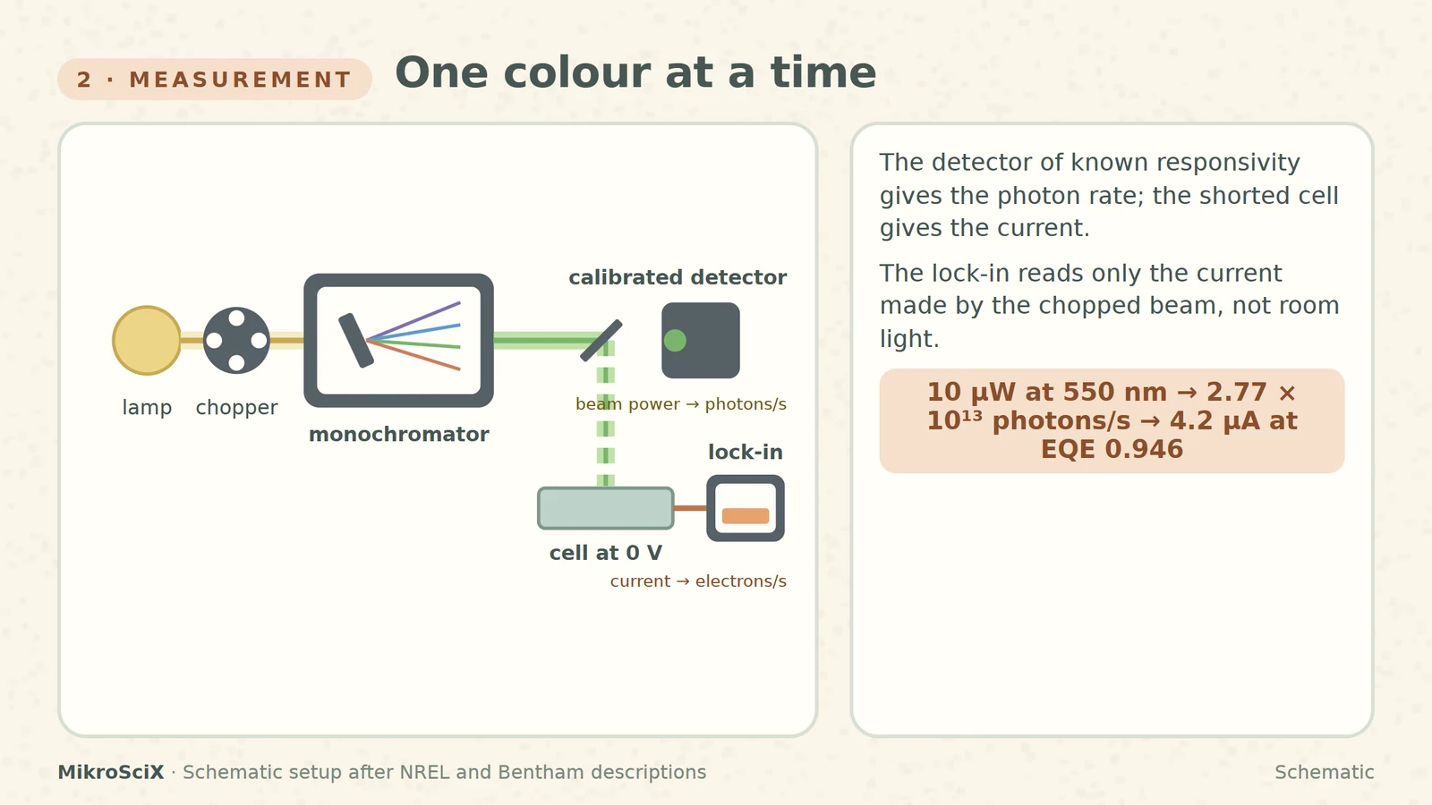
Check it yourself. The detector reads 10 µW at 550 nm. One photon carries hc/λ = 3.61 × 10⁻¹⁹ J, so the beam delivers 10⁻⁵ / 3.61 × 10⁻¹⁹ ≈ 2.77 × 10¹³ photons per second. With EQE = 0.946 the cell gives 0.946 × 2.77 × 10¹³ × 1.602 × 10⁻¹⁹ C ≈ 4.2 µA. The same answer from the responsivity: 0.42 A/W × 10 µW = 4.2 µA.

What breaks. A detector whose calibration does not cover the wavelength range; a reading taken without the chopper and lock-in, so room light adds current; and a cell that is not at short circuit.

3. Reading the shape: where the losses hide

An ideal cell would draw a square: QE = 1 for every photon above the band gap, 0 below it. Real curves sag in three places, and each place points to a different part of the cell [S1]:

• The blue end. Short wavelengths are absorbed very close to the front surface. If that surface recombines carriers quickly (poor passivation), the blue response drops.
• The whole curve. Reflection removes a slice everywhere. A low diffusion length in the bulk lowers the middle of the curve too, because carriers made there do not reach the junction.
• The red end. Long wavelengths are absorbed weakly and deep. Rear-surface recombination, weak absorption and low diffusion length all bite here. Below the band gap nothing is absorbed.

For silicon the gap is 1.12 eV, i.e. λ = 1239.8 / 1.12 ≈ 1107 nm. But silicon's band gap is indirect, so the curve does not fall off a cliff there: it slides down gradually as absorption gets weaker [S2].

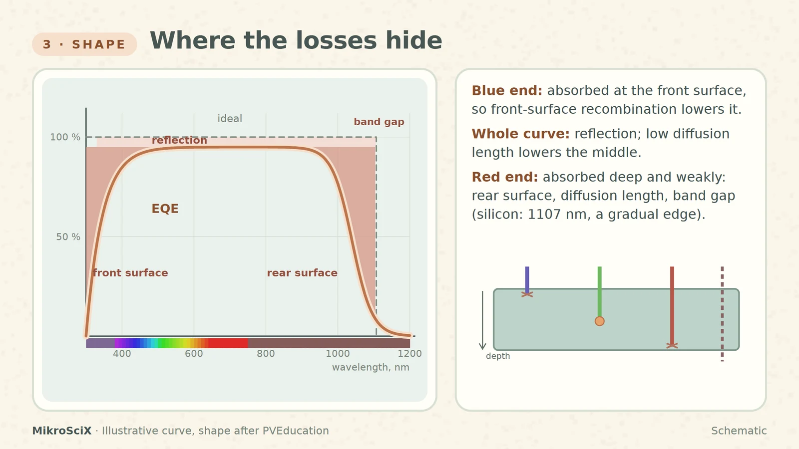
Check it yourself. A 1000 nm photon carries 1239.8 / 1000 ≈ 1.24 eV, above 1.12 eV: silicon can absorb it (our curve gives 0.77). A 1200 nm photon carries 1.03 eV: below the gap, so QE = 0.

What breaks. Blaming the blue loss on the bulk or the red loss on the front: depth decides which colour feels which surface.

4. From the curve to the current

EQE is electrons per photon. Multiply it by the number of photons the Sun sends at each wavelength and you get electrons per second at that wavelength. Add up over all wavelengths and multiply by the charge: that is the short-circuit current density [S4][S3][S5].

Jsc = q ∫ EQE(λ) · Φ(λ) dλ

Here Φ is the photon flux of the AM1.5G reference spectrum (ASTM G-173) [S6]. In a figure, the product is the area under EQE × photons.

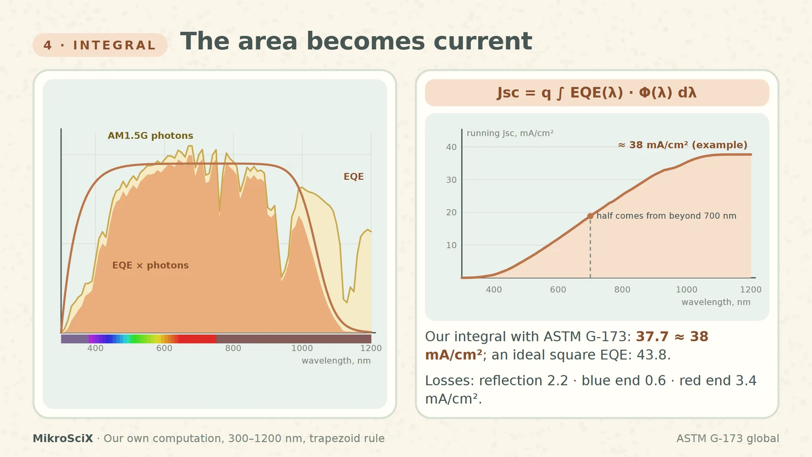
Check it yourself. We integrated our example EQE against the tabulated G-173 global spectrum from 300 to 1200 nm: 37.7 mA/cm², about 38. An ideal square EQE (1 up to 1107 nm) would give 43.8 mA/cm², so our example keeps 86 % of what silicon could collect. Taking the losses one at a time: reflection costs 2.2 mA/cm² (43.8 → 41.6), the blue end 0.6 (→ 41.0) and the red end 3.4 (→ 37.6, plus a little beyond the gap). One surprise from the running total: half of the current, 18.8 of 37.7 mA/cm², comes from light beyond 700 nm, so the red end matters as much as the visible.

5. A check on the solar simulator

The same Jsc can be measured directly from the J–V curve under a solar simulator. The two measurements are independent: the EQE route depends on the detector calibration and the reference spectrum, the J–V route on the simulator's intensity and spectrum. That is why comparing them is a standard consistency check, written into journal checklists; a large mismatch means something is wrong [S4]. It even works the other way round: one common way to set a simulator's intensity is to tune it until a reference silicon cell's J–V current matches its integrated EQE [S4].

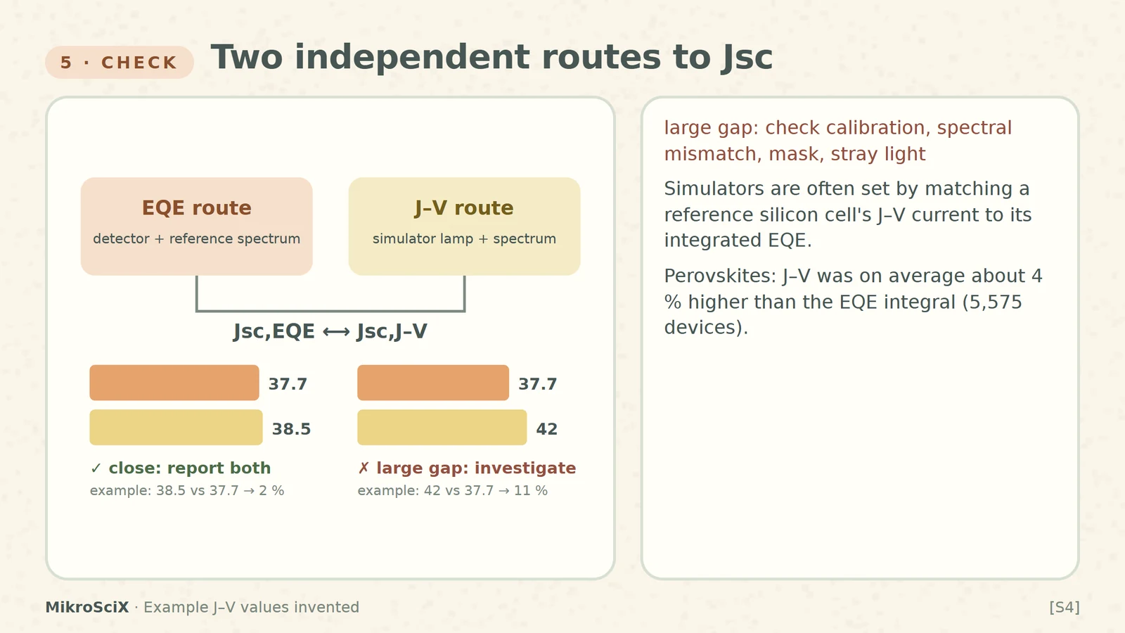
Check it yourself. The simulator J–V gives 38.5 mA/cm² for our example cell; the EQE integral gives 37.7. The difference is 0.8 / 37.7 ≈ 2 %: close. Had the J–V said 42, an 11 % gap, look at the lamp calibration, the spectral mismatch, the masking of the cell area and stray light before believing either number [S4]. (Both J–V values are invented.)

What breaks. Expecting a perfect match for every technology. In a database of more than 5,000 perovskite devices, the J–V value was on average about 4 % larger than the EQE integral and larger in over 83 % of cases; the reason is still open [S4]. There is no universal tolerance: state both numbers.

6. The one thing it is not: power efficiency

A cell with EQE near 100 % across the visible can still convert under a fifth of the light's power. Quantum efficiency counts electrons; power efficiency counts energy, η = Voc · Isc · FF / Pin [S7].

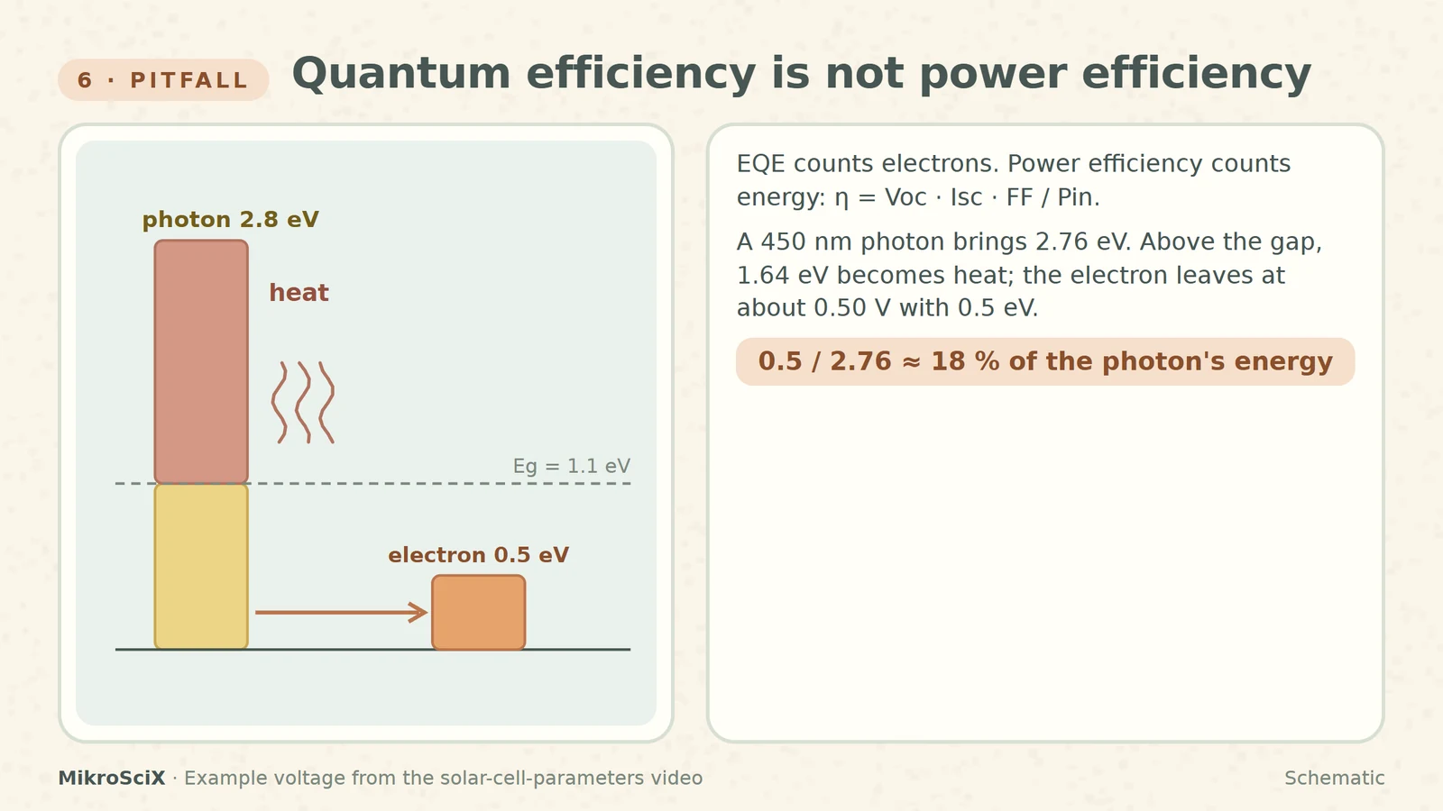
Check it yourself. A 450 nm photon brings 1239.8 / 450 ≈ 2.76 eV. Silicon keeps only about the band gap, 1.12 eV; the other 1.64 eV becomes heat as the carriers relax [S2]. And the electron does not even leave with 1.12 eV: delivered at about 0.50 V (the maximum-power point of the example cell in our solar-cell-parameters video), it carries 0.5 eV. That is 0.5 / 2.76 ≈ 18 % of the photon's energy, even though the photon was collected.

How to use an EQE curve

1. Read the shape first: blue end = front surface, plateau height = reflection and bulk, red end = rear surface and band gap.
2. Integrate it with the reference spectrum and compare with the J–V Jsc; report both.
3. Label it honestly: EQE or IQE, bias light or not, at short circuit or under voltage bias.
4. Never quote it as an efficiency: power needs voltage and fill factor.

EQE is a colour-by-colour photon count. Its shape tells you where the losses sit, its area tells you the current, and it says nothing about the voltage.

Try it yourself

1. 20 photons arrive, 2 are reflected, 15 are collected. EQE and IQE? EQE = 15/20 = 75 %; IQE = 15/18 ≈ 83 %.
2. EQE is 0.95 at 800 nm. What is the responsivity? SR = 0.95 × 800 / 1239.8 ≈ 0.61 A/W.
3. A new antireflection coating raises the whole curve but leaves the edges unchanged. Which number in section 4 shrinks? The reflection loss (2.2 mA/cm² in the example).
4. EQE integral 37.7 mA/cm², simulator 38.5 mA/cm². Is the simulator wrong? Not necessarily: about 2 % apart, a reasonable agreement; there is no universal tolerance, so report both.